home about telemetry projects publications gallery log

Time-nuttery 101

This post is meant as a layman's introduction to the insane rabbit hole that is time-nuttery — not so much the "why", as I think most time nuts have their own reasons for enjoying the field, but rather the "how". Perhaps my wife will understand why there is a Hydrogen Maser in the house...

Time

Time is sometimes quoted as being the SI Unit that can be measured to the highest precision. I am not quite sure I understand how to compare precision between units^[1], but there it is. Time is all around us and governs pretty much everything we do — but we cannot see it, nor interact with it in any meaningful way, and yet we can measure it with extraordinary precision. Fascinating stuff, but philosophy aside, precise time is vital to our society, in a very practical sense. The modern world would not be anything like what it is without our ability the measure time with high precision. For example, the modern electrical grid is depending on precise timing information in order to synchronise the various power stations. GPS would be conceptually unthinkable without high precision time — it is at the core of how it works. Forget about transmitting anything wirelessly. So, in addition to being cold, we'd all be lost as well. And we could not even post our misery on Facebook!

Grim prospects, indeed. Luckily, we do have the ability to measure time precisely^[2]. But before going into the measurement, let us look at the device usually tasked with keeping time, the humble oscillator.

Oscillators

Oscillators, or more precisely electronic oscillators in the more limited sense of interest to most time nuts, are funny little beasts. These little (or big) gadgets have only one purpose: To generate a varying electrical signal — over and over, again and again, very precisely. Just like an old grandfather clock^[3] that produces a tick and a tock, an electronic oscillator does the same thing, only with electricity. These things are in almost every electronic device we use, and it is getting quite hard to find examples of electrical appliances that typically does not contain at least one. Anything with a microprocessor, anything with a clock of any sort. Your cell-phone contains many, your microwave oven probably at least a couple.

The name of the game for the typical time nut is to measure and characterize the stability and accuracy of these devices. One of the properties of an oscillator is its frequency; how fast it ticks and tocks, how many ticks per second — measured in Hertz. A typical value might be 10 MHz, 10 million ticks per second. (They go into the billions of ticks per second.)

Time and frequency is related by the simple equation t = 1/f. The amount of time elapsed in one "tick" is equal to 1 over the frequency in Hertz. For a frequency of 10 MHz, each tick lasts 1/10 000 000 of a second, or 100 nanoseconds. In the world of time-nuttery 100ns is equivalent to about a week...

The "accuracy" of an oscillator is how close to the specified frequency it actually ticks — nothing is perfect, and if we look close enough there is always a little error. For an oscillator with a specified frequency of 10 MHz, the measured output might deviate by 1 Hertz — instead of 10 million ticks a second, it ticks 9 999 999 times. It is off by 1. Not a very accurate oscillator. For most practical purposes this may be of no consequence — in the course of a year, your wall clock would be off by a couple of seconds. But for other purposes it might mean the difference between a fast internet connection from your wireless device or no connection at all.

An oscillators "stability" on the other hand, is a measure of how its frequency change over time. If I measure the mentioned oscillator once more, it might tick 9 999 998 times per second. Now it's off by two. So it is not very accurate, and it's not very stable either.

Measurement

So, how do we go about actually measuring the accuracy and stability of oscillators? Well, somewhat simplified, we compare our Device Under Test (DUT) to some known (better) quantity, our Reference (REF), using some type of measurement device, commonly a frequency counter. We could count the number of ticks and tocks for precisely one second, and then we know the frequency. Plain and simple. This tells you something about the accuracy. Do it again and again, and you will know something about the stability.

Only... How do you know precisely how long a second is? This is where the reference comes in. The reference is your very best oscillator, that you trust to keep time to some specified uncertainty. A very small uncertainty. Within the walls of your lab, your reference defines how long a second is, or how fast 10 MHz is. If your reference differs from "true" frequency may or may not matter, it depends what you are interested in: A calibration laboratory is very interested in absolute accuracy, but a time nut may be more interested in stability.

The first lesson is that you never^[4] measure a single oscillator. You measure the combined instability of (at least) two oscillators; the DUT and the REF. If the stability and/or accuracy of the REF is known to be much better than the results observed, you can be confident that the measured instability is due to the DUT.

But... How do you know that the reference is any good? Well... You compare it to yet another other known quantity, an even better oscillator, with even less uncertainty. But even if you have done that, how do you know nothing changed since that comparison was made? How do you know that your reference is always as good as it was when you compared it last? Perhaps it is degrading, slowly developing a malfunction? Perhaps someone entered your lair while you weren't looking, just to tidy up a bit, and accidentally dropped your precious reference oscillator on the floor?

There is only one solution. You need another reference. One that is better, one that you can trust. You see where this is going, don't you.. About 5 minutes after the new reference is installed in the lab, the doubt creeps in: "Is this new reference as good as it is supposed to be? I must know!" Its turtles all the way down, you see.

Welcome. This is the entrance to the rabbit hole. You can leave your spare cash and time at the door, you will not see it again for some time...

Once this has happened a few times, you find yourself trying to explain to yourself, and pretty soon to your significant other, that you really do need a Hydrogen Maser.

Instrumentation

The reference is only part of the picture. Arguably the most important part, but still not the only part. Even given a "perfect" REF^[5], we still need some sort of instrument to carry out the comparison between the DUT and the REF.

There are a few instruments that could be used, but by far the most common is a Frequency Counter, or counter for short. Counters count the number of ticks occurring in a given time — the gate time. When the gate is closed, no measurements are taken. When the gate is open, the counter is doing its thing. A gate time of 1 second will count edges (ticks) for one second, and return an answer. Set the gate time longer, and the measurement will have higher precision.

The banner spec for frequency counters is the "single shot resolution" — the smallest increment of time it can discern. Older counters with a single shot resolution of 1 or 2 nanoseconds can be found second hand for a couple hundred dollars, less if you're patient/lucky. State of the art single shot resolution in a "general purpose" frequency counter is around 20 picoseconds. 20 picoseconds is a really, really tiny sliver of time — so tiny, in fact, that light itself can only travel about 6 mm in that time. I find that mindboggling.

The single shot resolution of the counter is directly responsible for the precision with which it can measure frequency. The "number of ticks in a second" is a little too simplistic — there is rarely a perfect integer number of ticks. So it needs to measure "partial ticks". Very simplified it measures the time from the gate opens until the start of the next "tick", and the last "whole tick" until the desired gate time has elapsed. From this, added to the number of "whole ticks" counted, it calculates what the frequency was.^[6]. Clearly, the higher resolution it can measure these "partial ticks" with, the more accurate the frequency measurement will be.

Incidentally, this is also the reason why a longer gate time gives better precision — the counter only counts two "partial ticks", the first and the last. The limited resolution of the "partial ticks" plays a smaller and smaller part as the number of "whole ticks" gets larger.

Software

There is still a piece of the puzzle missing; a good reference and an instrument that meets your requirements (or budget) is not enough to get much insight — you also need software to carry out the analysis. While it is very possible to create such software yourself, some people prefer a readymade solution. The "industry standard" for analysis is Stable32, which is now freely available from IEEE. This program is very thorough in its analysis-capability, but you need to feed it a datafile with frequency or phase measurements — so actually collecting and storing the measurements is left as an exercise for the user. TimeLab, on the other hand, while a bit lighter on the statistics, is able to collect readings from a wide variety of frequency counters "out of the box". Keep in mind that Timelab does not configure the instrument, it merely collects the readings. You must set up the frequency counter correctly prior to starting an acquisition.

Also very much worth mentioning is a collection of small utilities by Tom van Baak — my personal favourite is da. Read the source code (the .c-files) for a short description of what each utility does.

Frequency and Phase

When I started this hobby, phrases such as "phase record" and "phase measurements" floated around a lot. It took too long before I understood what turned out to be a very simple concept, so I will explain my understanding here — to the presumed joy and universal acclaim of thousands of frustrated would-be time nuts.

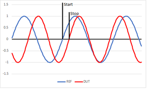
The concept of frequency is easy enough: How many ticks does the DUT produce, per second as defined by the REF. The concept of phase is almost as easy: Imagine you start a timer on an edge (a tick) from the Reference. Then, stop the timer on the first edge that follows this from the DUT. There. You have made a phase measurement. For 10 MHz oscillators, the measured value can be anywhere from 0 to 100 nanoseconds. This is also referred to as a Time Interval measurement, and the Single Shot Resolution of your counter dictates the precision with which measurements are made. Commonly, the REF is divided down so that it produces one tick every second, and we therefore make one measurement per second. But this particular cat can be skinned many ways.

A single phase measurement tells you very little. But if you make another one, you can tell how much the DUT differs from the REF — if the measurement is the same, they are ticking along at the same frequency. If not, you can calculate the difference in frequency.

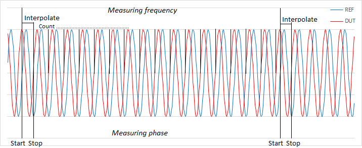
Worth taking a moment to think about is the difference in measuring frequency and measuring phase, which I have attempted to illustrate in the plot on the left. In order to measure frequency, we must observe every tick the oscillator produces. This is a bit of a challenge, as most counters will typically introduce what is known as "dead time", or gaps in the measurements. When the frequency counter is busy reporting the last measurement, it is not taking a new measurement. This is suboptimal, because it introduces errors, "bias", in the measurements. How big an issue this actually is, is up for debate. Modern counters are capable of making gap free measurements, but we need not shell out thousands of dollars to avoid dead time.

If the REF and the DUT are pretty stable, and their frequencies close to each other, we can be sure that by measuring the time interval between the start edge from the REF and the stop edge from the DUT, we have not missed anything. The observation interval must be short enough that we are confident we won't miss a complete tick in the meantime. If there was one very short "tick" somewhere in the interval, we would observe that in the following time interval measurement — we sort of measure the "average frequency" of the DUT for one period. Which is precisely what we seek to measure. If we want to know if there are short or long ticks in there, we must measure these using shorter observation intervals. Note that the REF and DUT does not really need to be the same frequency, but they must divide evenly. In practice this is rarely an issue, since for precision oscillators, by far the most common frequencies are 5 and 10 MHz.

Here is an important mental leap to make. Phase and frequency are two sides to the same coin — two ways of measuring the same phenomenon, the oscillations coming out of the DUT. Phase is the "integral of the frequency" — if the frequency change we will see that clearly on the phase measurements — frequency of the DUT goes up with respect to the REF, the time interval will go down. An offset in frequency leads to a slope in phase — which makes sense; if the DUT ticks slower than the REF, the time interval between a rising edge from the REF and the rising edge from the DUT will become longer and longer. Even tiny differences which would all but disappear if we measure frequency directly, will be plainly visible if we measure phase — given enough time.

We can trade time for precision when measuring frequency as well. Each individual reading can not be improved upon, but by taking lots of readings and averaging them, we get closer and closer to the "true" frequency of the DUT. The phase record (the plot of all the phase measurements taken), however, quite often gives some additional insight into what is going on with your measurements — you can see its development over time. In particular, temperature changes will be very visible. (And annoying.)

An analogy for the relationship between phase and frequency might be two cars driving on a circular race track. One car is our Reference — it drives at precisely 10 km/h. The other car is our DUT; it drives at close to 10 km/h, but we do not yet know how close. We could measure the speed of the DUT when it crosses the start/stop line. This is analogous to measuring Frequency. No measurement is without noise, and for this analogy let's say we can measure speed with an accuracy of 0.1km/h. We will have to average many measurements before we know with precision what speed our DUT keeps, or if it is lagging or leading the Reference car.

If, on the other hand, we measure the difference between the two cars at the start/stop-line, the picture changes slightly. We can measure the time (or distance for that matter, but let's stick with time) from the Reference-car passes the line, until the other car passes the same point. This is analogous to measuring phase. It is easy to see that this number will be steadily growing (or shrinking) by each lap, even if the difference in speed is slight. Likewise, if the speed of the two cars is precisely the same, this number will be stationary. The amount of noise in the measurement will be the same, though.

This also brings us on to another irksome fact of measuring phase — what happens when, after many laps, one car leads by a full lap? In the last lap, the REF was leading by let's say 59 seconds, but in this lap it is only leading by 1 second. This is what's known as a "phase wrap" — when one oscillator "overtakes" the other by a full cycle. It can be dealt with a couple of ways — you can divide down the signals to make the "lap longer". But it is easy to spot in the phase record, and easy to correct; you just add one complete "lap" to the measurement. In our example, this would be however long our Reference-car takes to complete one lap, or "cycle". For a 10 MHz oscillator, one cycle is 100 nanoseconds. TimeLab and Stable32 can handle phase wraps, da.exe can also be used to "unwrap" a phase record.

Hopefully it is easy to see how a change in speed (our standin for frequency) translates into a change in phase - they are not independent quantities, you can not change one without affecting the other.

Keep in mind that this is an analogy — don't think too hard about it, or it will break.

Another term that shows up, particularly when reading scholarly papers on the various deviations and variances that can be used to gain insight into the characteristics of oscillators is "fractional frequency", often denominated y(t). This is nothing more than "the measured value divided by the expected value minus 1". The expected value is basically what the label on the oscillator says^[7]. As an example, say we measure 10 000 000,02 Hz from a supposedly 10 MHz oscillator. The fractional frequency is (10 000 000,02 / 10 000 000) - 1 = 2e-9. The advantage is that we can compare frequency offsets between oscillators of differing nominal frequencies, similar in concept to "percent". The term x(t) is often used for "Phase measurement at time t".

You can convert between phase and frequency, sort of. Technically, a phase record on its own can never tell you the actual frequency you are measuring. It can only accurately describe the difference between the REF and the DUT — and even with this more limited statement, there's a gotcha. Imagine you have a 10 MHz reference, and set up a time interval measurement between a Pulse Per Second (PPS), derived from your REF, and a supposedly 10 MHz signal from your DUT. Further, imagine that the 10 MHz DUT is does not in fact chug along at 10 000 000 Hz, but rather 10 000 001 Hz. How would that look to the counter? Identical, that's how. In practice, we already know roughly the frequency, we seek to measure tiny differences from the nominal frequency. So it is not really a problem, although some care must be taken.

Regardless of choice of measurement, if you want to gain some insight into how the DUT behaves over time, you need to collect data over time. Lots of time. Once the data is collected, it needs to be analysed, which brings us on to...

Lies, damn lies, and statistics: Allan Deviation

The accuracy of an oscillator does not really require any fancy mathematics, at most some averaging. It differs by some small amount from your reference, and that number is pretty much the end of the story — given that the Reference is your local definition of frequency.

When we discuss stability, though, it is not quite as simple. Stability^[8], as mentioned, is how the frequency changes over time. We need some convenient way to assign numbers to this property. What we have to work with is a time series of phase or frequency measurements, taken at regular intervals. This interval is commonly referred to as tau^[9], and if you are measuring frequency using a frequency counter, it is equal to the gate time.

As a first attempt, it may be tempting to use the Standard Deviation. After all, it is a measure of "how diverse", or how spread out, a dataset is — which would be a measure of stability. If the DUT is very stable at the intervals observed, all the frequency measurements would be close together, and the standard deviation would be small. Chop up the list again and again, averaging as required, to get some insight into how stable the DUT is in multiples of tau timescales.

As an example, assume we make frequency measurements with a 1 second gate time — tau is 1 second. Take the standard deviation of the complete list, and we can say something about how stable the DUT is from one second to the next. But we also want to know how stable it is on two second intervals, or 10 second intervals or 100 second intervals. No problem. Take two consecutive measurements and average them. Do this through the whole list and calculate the standard deviation again on the resulting list. We now know how it behaves at tau 2 seconds. Repeat the same process for any time interval needed. Finally, plot the resulting values, and you know quite a bit about how the oscillator behaves at various timescales. Plot it on a logarithmic scale, so that we can look at the very small at the same time as the very large.

Conceptually, this is what calculating Allan Deviation (or Allan Variance; ADEV = Sqrt(AVAR)) does. Only not quite. The standard deviation does not converge in the presence of some noise types commonly observed in oscillators — basically, the value we get as we average larger and larger chunks of data depends not on the amount of noise present in the data, which is what we seek to quantify, but rather on the number of datapoints averaged. Clearly this is not good enough, and in 1966 David W. Allan came up with a solution: The Allan Deviation, ADEV for short. ADEV does calculate the standard deviation, but it "massages" the frequency or phase record before operating on it. Several other deviations have been proposed since, but ADEV is the most common. Another worth mentioning is the Modified Allan Deviation, MDEV. Conceptually similar, it is better at separating some noise types — more on that later.^[10]

Looking at the plot, it is important to realise that the value at the 10 second marker on the x-axis does not say anything about "what the oscillator did 10 seconds into the measurement", but rather "how different two frequency measurements taken 10 seconds apart can reasonably be expected to be". It is a result of hundreds or thousands of datapoints, all spaced out with 10 seconds between them. To know what the oscillator did at any given point in the measurement, you must consult the phase or frequency plot.

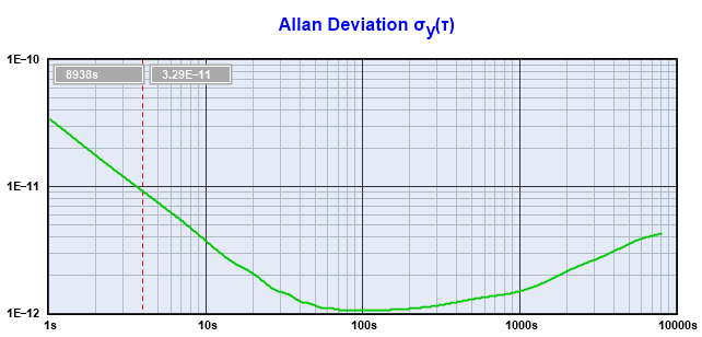
For example, an Allan Deviation of 3.5e-11 at tau 1 second should be interpreted as there being an instability in frequency between two observations a second apart with a relative root mean square (RMS) value of 3.5e−11.

The plot on the left actually tells us two things: It does say a lot about how stable the DUT is on any timescale measured, but it also says something about the types of noise present in the data.

Types of noise

Somewhat alien in concept to the uninitiated, noise comes in different flavours. The easiest to understand is what is known as "white noise". Let us use a die (dice?) as an example. The "expected value" of a throw is the sum of 1+2+3+4+5+6/6=3.5. Obviously, you will in fact never throw 3.5, but on average over many throws, it is easy to see that you should end up with this value. Each throw will give one of the 6 values, and assuming the die is fair, no value is more likely than another. The value you get is also not depending on what value you got on any previous throw.

Throw such a fair die 100 times and tabulate the result. Start adding up and taking averages: Add groups of two and divide the results by two. Add groups of three and divide the results by three. Pretty soon you will see that you are getting closer and closer to the expected value of 3.5.

In fact, the standard deviation of your averages will be proportional to 1/square root(N), where N is the number of samples in the average. Therefore, the more points are taken in each average, the smaller the standard deviation from the average. In other words, the more points averaged, the closer you get to the actual value. Average 100 values, and your standard deviation is 1/10th of the individual errors. Average 625 values, and your error should be 1/25th. Over a sufficiently large dataset, that is.

This holds for White FM, or white frequency-modulated noise. Looking at the plot below, we see a section that has a slope of -.5: Two decades over (i.e. x100 averages, logarithmic remember), and one decade down (sqrt(100) = 10). Other noise types are not quite so easy to describe. The slope of the ADEV plot shows how the dominant noise form "behaves" under averaging as the number of averages increase.

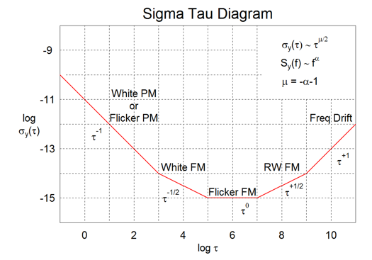
The various noise types distinguished by ADEV and their associated slopes are seen in the plot on the right:

An important difference between ADEV and MDEV, is that MDEV is able to distinguish between White PM and Flicker PM. The slopes are also different for other noise types.

It's a bit tricky to get to terms with these different noise types — what are they anyway? Suffice it so say, the slope identifies the dominant noise types, which can tell you something about where the noise is coming from. The leftmost portion of the plot, for instance, is revealing: A slope of -1 is White PM (Phase Modulated), a tell-tale sign of quantization noise. This part of the plot is dominated by the resolution of the frequency counter used — and the level of the slope tells you what the single shot resolution of the counter is. A level of 1e-9 at tau 1 second = 1 nanosecond. Of course, there are many ways in which to screw up a measurement such that other noise than quantization noise dominates...

An important point to note is that the portion of the plot dominated by noise in the instrumentation tells you nothing about what the oscillator is doing — even the best reference in the world will do nothing to bring this part of the plot down. So if you are measuring very stable oscillators, the amount of the plot that is obscured by instrument noise becomes an issue — for a 1 ns counter, in order to measure a really good oscillator that has an ADEV of 1e-13, you need to average over 10 000 seconds... You get no insight into what the oscillator is doing over timescales less than 10 000 seconds. It also means your actual measurement time would be a quite a bit longer — keep in mind we need to compare a lot of 10 0000 second intervals before we can have confidence in our measurements. (Thankfully, ADEV is usually calculated using overlapped intervals — so it is not quite as bad as it sounds.)

On the other hand, if you measure the same oscillators with a 20 ps counter, you would get to 1e-13 in about 200 seconds. Which explains why counters with good single shot resolution are in demand. MDEV also has an edge over ADEV in this regard — white PM has a steeper slope in MDEV, so we get to the "interesting bits" faster when we use MDEV.

...but what time is it?

So far, we've considered the precise measurement of time intervals — how long is a second, any second. But there is also the need to know when an event took place, in a more global sense. A very precise, very stable oscillator can tell you how long a second is, but it won't tell you what time it is. For this you need a clock. A clock is simply an oscillator coupled with a counter: The oscillator produces carefully timed ticks (pulses) at a known rate, and the counter counts how many pulses it has seen. Continuing the example of a 10 MHz oscillator, after the counter has counted 10 million pulses, the clock knows a second has passed. Add this second to whatever the clock already thinks the time is, and we are all good. Except... How do we tell it what time it is in the first place?

A branch in the rabbit hole. Well, we can try to get time from some known source, the internet perhaps. We can rig up a computer to fetch "true time" from some reputable source on the internet, and tell the counter the initial time before it starts counting pulses — we set the clock. That will get us reasonably close, to within a few milliseconds of "true" time. There are lots of stuff between your computer and wherever your get the time from, all adding an unknown amount of delay, and not all of it can be calibrated out. This is how most computers are kept roughly on time. But milliseconds... That's really not something to brag about, is it? No, it is not. Not at all. Well, for most practical purposes, a millisecond or two is of little consequence, but we are time nuts. Milliseconds are right out, even microseconds are for the feebleminded. No, we want nanoseconds at the very least, and picoseconds if we can get it!^[11]

But before we can get to picoseconds, an excursion into what "true time" means is in order — it is not as simple as it sounds. In ye olden days, it was simple. When the sun is directly over head, it is noon. Set your clocks to 12:00:00, and we'll go from there. For most human endeavours, this was quite good enough. Until trains came along, that is. The sun might be directly over head in London a good few minutes before it is directly over head in some other station on the line. So how do you work out the train tables? Which time, as it were, will be printed on the timetables? Navigation at sea, once clocks accurate enough were available, also required some agreed upon timescale.

Clearly, a national time standard was required. That is a pretty long story, which can be read about elsewhere, but in the end England, and much of the world with it, settled on "Greenwich Mean Time". The challenge, which pretty much remains the same today, is this: If, at Greenwich, they know by definition precisely what time it is, how do you "transfer" this knowledge to somewhere remote? In the early days, this was done by physically taking several "travelling" clocks from wherever precise time was needed to the Royal Observatory in Greenwich, and setting the clocks there. These clocks, "transfer standards", were then brought back and used to set the local master clock.^[12]

Even after the adoption of atomic time in 1967, the challenge remains pretty much the same. And for years the solution was the same as well. Caesium Beam Tube clocks were travelling on commercial airlines to and from various labs to be calibrated and set. It was only after satellites came along that this practice ended.

"What time is it" is a reasonable question to ask, but it looses its meaning then the precision of the answer is in the nanoseconds. When you are done reading the answer, it is no longer correct. Often, a more productive question to ask is "what time was it"; when did an event take place.

...all right, what time was it

If you and me both take our radio astronomical observatories out from under the stairs, set them up in the back yard and agree on a quasar to observe, we could do some interesting things from our knowledge of the precise time at which the signals arrive at each location.

This technique is called Very Long Baseline Interferometry, VLBI, and radio observatories were the first "commercial" users of Hydrogen Masers — they were constructed specifically to their requirements. EFOS-3, for instance, lived most of its life at the Wettzell observatory in Germany.

Note that each of us having a really precise and stable oscillator will not be sufficient — if you observe an event at 12:00:00 according to your clock, and I observe the same event at 12:00:01 according to my clock, unless our clocks are synchronised we will not know the difference in arrival time of the radio waves constituting the observation. Which is the whole point. Except... If we are both able to compare each of our clocks to a third clock, simultaneously, we will know the difference between our clocks. Then it is simply a matter of subtracting the differences, and we have a common timescale that will allow us to work our magic on the observations. Crucially, this third clock need not be very accurate, as long as we both observe it at the same time. When we subtract the differences, the third clock "falls out of the equation", so to speak.

This is known as a "paper clock". It does not really matter if my clock is off by some amount from "true time" (whatever that is), as long as I know by how much. I do not even need to know by how much now, as long as a record is kept. Then we can both go back to our observations long after the fact, correct the timestamps on our observations and do our calculations.

This is pretty much how the "world time scale" TAI^[13] (International Atomic Time) is kept. TAI is the product of tens of national time laboratories, and a few hundred atomic clocks — but counterintuitively, none of the clocks are "correct". The differences are tiny, in the nanosecond and picosecond range, but the fact is that none of them has the "correct" time at any instant. It is calculated after the fact. The participating time laboratories are comparing their clocks to other laboratories' clocks using satellites and other means continuously. Once a month, all these records are compared, and an average is computed. Then, from this each laboratory can calculate how wrong each clock was at any point in time in the past month.

Timescales; UTC, TAI end friends

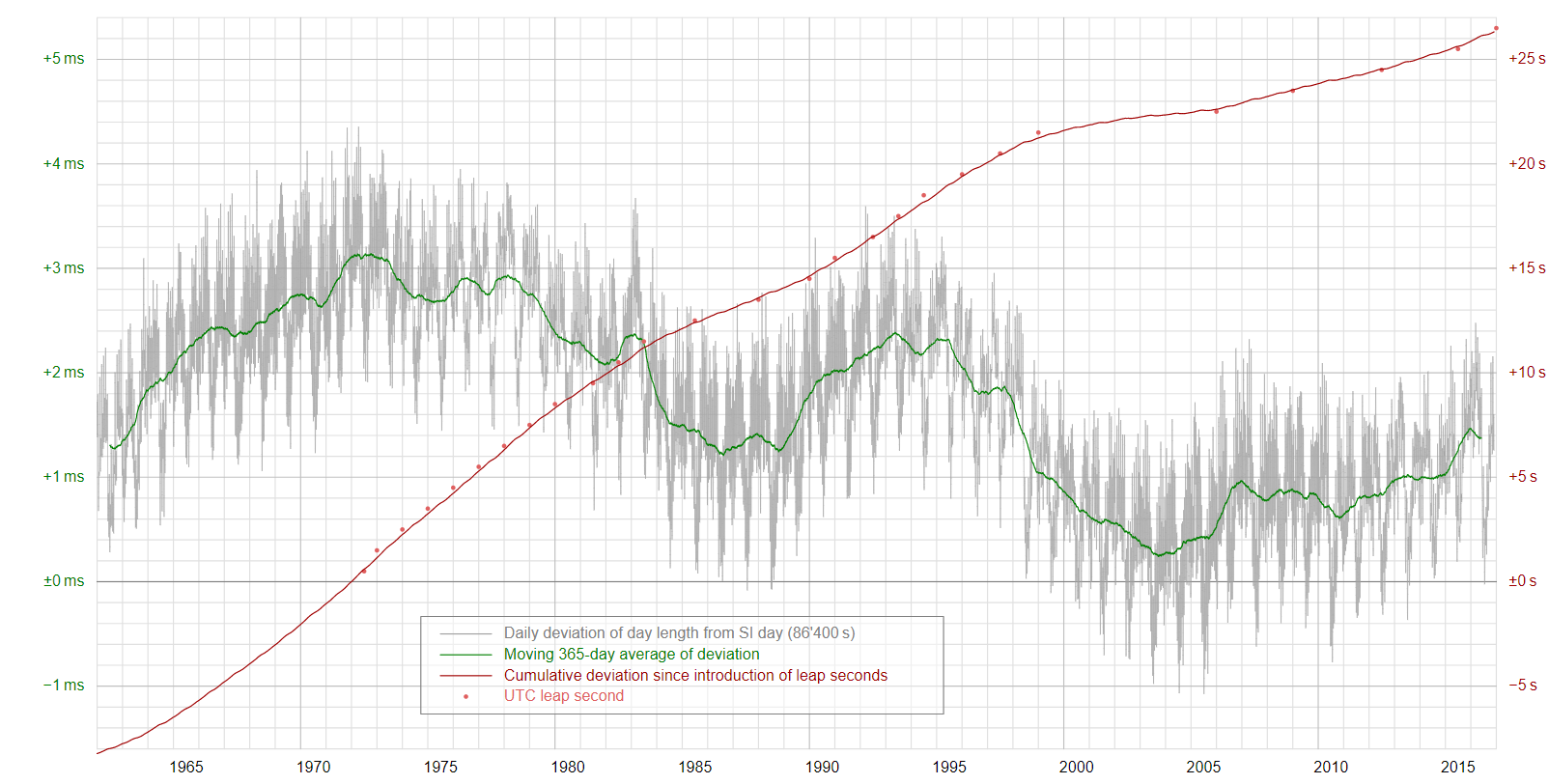
Asking what time it is, or even was, is well enough. But according to who? In the beginning, noon meant "the time at which the sun is directly over head". Later, it became, "the time at which the sun is directly over head at some specific location". It soon became evident that the earth is a pretty poor timekeeper — each revolution does not take precisely the same amount of time every time, the duration of a day changes by as much as a few milliseconds^[14]. Using the "sun directly over head", or other astronomical observations, as an indication of time was not sufficient. Thus atomic time was adopted.

The concept of using atoms to keep time has been floating around since it was suggested by Lord Kelvin in 1879. The first accurate atomic clock was built in England in 1955, by Louis Essen and Jack Parry at the National Physical Laboratory. It was based on a certain transition of the Caesium-133 atom. Then, in 1967, the International System of Units (SI) defined the second as "the duration of 9 192 631 770 cycles of radiation corresponding to the transition between two energy levels of the Caesium-133 atom." Now you know.

With atomic time, we know with great precision how long one second is. And by definition, a day is 86400 seconds long. The problem is that the earth does not play ball — it rotates in its own sweet time, Caesium atoms be damned. And that time is slowing down. Consequently, if we were to adhere strictly to TAI, 12 o'clock would eventually no longer happen when the sun is approximately directly over head. 12 o'clock might, some time in the future, happen at sunrise! Clearly, not what we want. So, in order to keep noon and 12 o'clock happen roughly at the same time, we add leap seconds to TAI when we need to. The result is what we call UTC, Coordinated Universal Time

There are many other timescales around, some of which are of interest primarily to smaller groups such as astronomers, but at least GPS time should be mentioned. GPS relies on a very precise, global timescale, that everyone at the party agree to; the satellites, the receivers, and the ground stations. The system is not really concerned with the concept of "noon", though, so as long as everyone agrees to the same timescale, it does not really matter what that time scale is. GPS time is not UTC, nor is it TAI. GPS time is kept by the US Naval Observatory, but conveniently it is steered towards TAI — a new second in GPS time starts at roughly the same instant as a new second in TAI. GPS time is off by 19 seconds compared to TAI, though. And TAI itself is off from UTC by the number of leap-seconds currently added.

The story is of course longer and more convoluted than this, though. The rabbit hole goes deeper. Much, much deeper.

Gas, Rocks and Metal — Different Types of Oscillators

There are many ways to build oscillators, depending on what feature is most important: Price, size, accuracy, stability, insensitivity to environmental factors... The list goes on. For time nuts, though, accuracy, and perhaps even more, stability is of prime concern.

The first really accurate electronic oscillators were made from quartz. Quartz has a peculiar property in that it is piezoelectric — give it some juice, and the quartz crystal physically contracts. Likewise, give it a squeeze, and it produces a small electric charge. This was cleverly used to make pretty good oscillators from the 1920's onwards^[15]. Quartz is still the most common material to craft oscillators from, although solid state MEMS oscillators are rapidly gaining ground.

Quartz oscillators may be common as gravel, but quartz can also make for some of the best oscillators money (a lot of money) can buy — at least when viewed over short time spans. Most atomic clocks in fact contain a quartz oscillator that is controlled, or "disciplined", by the atomic phenomena exploited to gain good longer term stability.

Speaking of atomic clocks, this might be a good opportunity to introduce the most common types — the types you could conceivably order from a manufacturer, had you recently won the lottery. I must confess to some laziness here, the descriptions and diagrams are largely lifted from NIST's "Time and Frequency from A to Z".

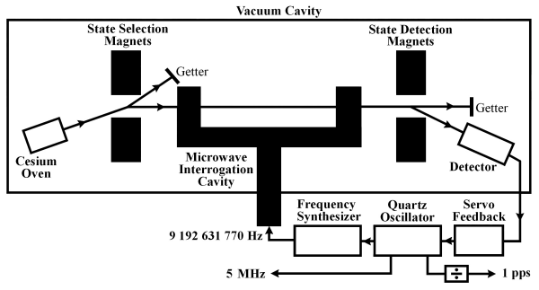
The first type was the first atomic clock successfully used to measure time — the Caesium Beam Tube. In a CBT, a small amount of Caesium is heated to a gas in an oven. A hole in the oven allows the atoms to escape at high speed into a high vacuum, magnetically shielded chamber. The atoms then pass between two strong magnets which causes the atoms to separate into two beams, depending on which spin energy state they are in. Those in the higher energy state are discarded, while those atoms in the lower energy state are exposed to a radio frequency field, the frequency of which is derived from a quartz oscillator in the instrument. The absorption of this RF energy excites many of the atoms from the lower to the higher energy state. The beam continues through another pair of magnets, whose field again divides up the beam into high and low energy states. Those atoms in the higher energy state are sent to a detector.

The number of atoms that are detected in the high energy state is a direct result of the frequency of the RF field. If the frequency of the RF field is too high or too low, the field will not excite the atoms into the high energy state. This is the "interrogation mechanism" — the quartz oscillator that produces the RF field is electronically tuned such that the number of atoms in the high energy state is maximised. We now have our very precise frequency.

While the Caesium clock was the first successful atomic clock, the first atomic clock to be built was in fact a maser — an ammonia maser, in 1949. It did not work particularly well. While the Caesium clock went on to define the second, its short term stability is actually not very good — if you measure it over days or weeks, the average frequency will be extremely accurate. But if you measure from second to second, it's really not that great. A few years after Essen built his Caesium clock, the first Hydrogen Maser was constructed in 1960 by Goldenberg, Kleppner and Ramsey. Subsequently, masers found use with the new technique of VLBI. The Hydrogen Maser has vastly improved short term stability over the Caesium Beam Tube, but it has a few quirks that makes it less suited for long term time keeping. Several masers nevertheless contribute to TAI.

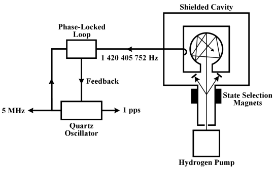
A hydrogen maser works by sending hydrogen gas through a magnetic gate that only allows atoms in certain energy states to pass through. The atoms that make it through the gate enter a storage bulb surrounded by a tuned, resonant cavity. Once inside the bulb, some atoms drop to a lower energy level, releasing photons of microwave frequency. These photons stimulate other atoms to drop their energy level, and they in turn release additional photons. In this manner, a self-sustaining microwave field builds up in the bulb. The tuned cavity around the bulb helps to redirect photons back into the system to keep the oscillation going. The result is a microwave signal that is locked to the resonance frequency of the hydrogen atom and that is continually emitted as long as new atoms are fed into the system. This signal keeps a quartz oscillator in step with the resonance frequency of hydrogen, as shown in the figure.

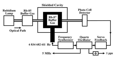
Finally, the last commercially successful atmomic clock is also the most common. It can be picked up surplus from the telecom market for a modest price. The Rubidium clock.

Rubidium oscillators operate near 6.83 GHz, the resonance frequency of a specific isotope of the rubidium atom (Rb87), and use the rubidium frequency to control the frequency of a quartz oscillator. A rubidium lamp containing Rb85 and Rb87 is excited to a glowing state, and the optical beam excites Rb87 buffer gas atoms into a particular energy state. Microwaves from the frequency synthesizer induce transitions to a different energy state. This increase the absorption of the optical beam by the Rb87 buffer gas. A photo cell detector measures how much of the beam is absorbed and its output is used to tune a quartz oscillator to a frequency that maximizes the amount of light absorption. The quartz oscillator is then locked to the resonance frequency of rubidium, and standard frequencies are derived from the quartz oscillator and provided as outputs as shown in the diagram.

These are by no means the only atomic clocks in existence, but they are the most common ones commercially available.

The Measurement of Time: Time, Frequency and the Atomic Clock	Covers very broad spectrum of measurement techniques, analysis of results, and history. My favourite.
The Quantum Beat: Principles and Applications of Atomic Clocks	Covers much of the same as The Measurement of Time, I found it a bit heavier going at times — but certainly a "must have" if that book leaves you wanting more.