Using Precise Point Positioning for stability measurement of stable oscillators
I've been tinkering with a setup to use PPP to measure the stability of my Hydrogen Maser. After much flailing, I have decided to write it up on this webpage, to perhaps save someone else some of the confusion I have had trying to make this work. It is really rather straight forward, but I never found a simple, step by step explanation of the process.
Preliminaries
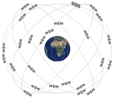
If you know the exact position in space and time a signal originated in, and you know the precise time when the signal was received, you can calculate the distance between the receiver and the transmitter. If you have at least four such signals, you can calculate your precise position. In two sentences, this is how GPS works - there are numerous websites diving in to the details, so I will stick to the broad strokes.
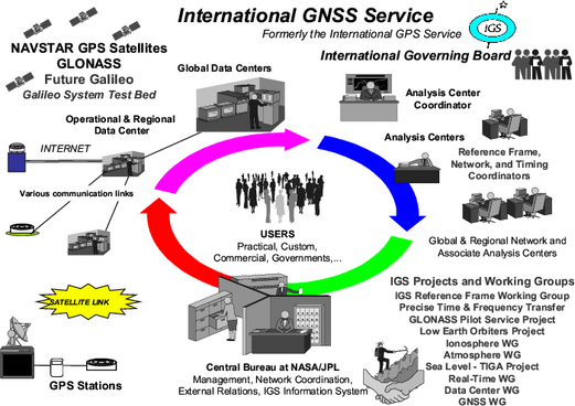
But how do you know each satellites exact position, and for that matter the precise time the signal was transmitted? The satellites has a model of its own position in time and space, and encode this information in the signal sent from the satellite. The model the satellite has, while very good, is still limited - it is only a model. So IGS and other agencies measure both the precise orbits of the satellites, as well as the on-board clock accuracy using networks of ground receivers. The corrected clock and orbit information is available as "precise clock products" and "precise orbits".
Precise Point Positioning is a method of combining the observations made by the GPS receiver with the precise corrections from IGS or other agencies, giving a much more precise position than what is obtainable using the information broadcast from the satellites. The PPP process also gives a very precise measurement of the GPS receivers local oscillator, which is what is of interest to the average time-nut. The process is "after the fact" - as with many things of interest to time-nuts, it requires a not insignificant amount of patience. In short, measurements made one day will not be available untill the corrections are ready some time in the future. (There are some ifs a buts to this, but in general this is the case)
The IGS collects observations from several Analysis Centres - 12 the last time I looked. The ACs also release their own products, but the official corrections are released by the IGS, and is a weighted average of the corrections from the different ACs. Statistics and comparisons of the individual ACs products are available at the IGS website here. The ACs have different strategies to analysing their products, which can be found here.
The IGS products come in several flavors; "Ultra rapid", "Rapid" and "Final".
- "Ultra rapid" is available several times per day, and contains a mix of the previous days observations, and a forecast for the next 24 hours. The least precise of the three.
- "Rapid" is made available roughly 17 hours after the previous GPS day. Contains precise measured orbits and clocks for a 24 hour observation window. I will use these corrections in the example.
- "Final" is available several days after the observations are made. These are the most precise corrections available, but in practice the Rapid products are good enough.
Several types of corrections are made available, but for this use we only need two: the precise orbits, available in .sp3-files, and the precise clock corrections, available in .CLK-files. (For Ultra-rapid, only .sp3-files are available. The naming also includes an additional hour field.)
I want to mention that the .sp3-files do indeed contain clock corrections, but the corrections are only given at 15 minute intervals. The .CLK-files contain corrections given at 5 minute intervals. (For the Rapid products.)
The naming of the corrections is a bit involved. In addition to the extensions already described, the filenames starts with "igu" for IGS ultra rapid, "igr" for IGS rapid, and "igs" for the final products. Other ACs have other combinations. Then follows the four digits GPS week the corrections are for, and one single digit describing the day of the week. So, for Saturday October 28th 2017, the Rapid clock-products will be called "igr19725.CLK" - IGS Rapid clock product for day 5 of GPS week 1972. Here is a good calendar showing GPS weeks and days.
The corrections are available a couple of places, but I get them from CDDIS' ftp-site.
This all sounds well and good, but where to start? Turns out, it is a pretty painless process, at least if frequency is the primary interest. If precise time, and by "precise" I mean "within tens or hundreds of picoseconds", is the primary interest the process becomes a bit more involved. Personally, frequency is what I am interested in - I want to know that my oscillators are stable, I don't particularly care if the phase of each "tick" is a few nanoseconds different from TAI. National timing laboratories care - but they have PhD's who know these things.
First and foremost what is needed is a "geodetic GPS receiver" - I have not seen a definition for what the term means, but what is needed is a GPS receiver that has the following features:
- Must be able to take an external reference.
- Must be able to report code and phase pseudorange observations. (I.e. it must be possible to somehow get a valid RINEX observation-file from the reciever.)
- It must be dual frequency - it might be possible to use the process on a single frequency receiver and some sort of precise ionospheric maps, but I have not tried.
Professional grade survey receivers have many, many more options than this. But what we need are the raw pseudorange measurements. How the receiver calculates a position, sends or receives differential corrections to/from other receivers, position hold mode, PPS out or not - all of this is irrelevant for our use. (Well, PPS out might come in handy..)
Features that may be worth considering for future use is the ability to track L2C, L5 and GLONASS. These features are not required to get good results at present, but if a receiver can be had that has these features, I'd take them. But I would not pay a lot of money for them (again..), but that is just my opinion. Antennas that can handle L1/L2/L5 GPS and GLONASS are also harder to find surplus.
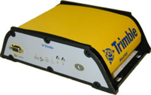
I've tested, and I continously run, both a Trimble NetRS and a Novatel OEMV-3 and they both work well. Presumably numerous other recivers will work as well. If I were to give a recommendation I'd lean towards the NetRS, for two reasons: (1) it logs observations to internal storage, so rebooting the host computer does not interrupt the measurements, and (2) the observations can be logged in a format that can directly be read by teqc.exe - which simplifies the post processing a bit. It also has an ethernet interface, and they show up fairly regularly on eBay for an acceptable price. I will use the Trimble as example in this post.
I do not see much difference in the results between the Novatel and the Trimble, if anything I think the Trimble might have a bit less noise. The Novatel, on the other hand, has much more flexibility in how it can be configured, and it might be possible to tweak the setup to match or exceed the NetRS. The difference, if it exists, is slight though.
Regardless of the receiver chosen, antenna quality and placement is also very important. A professional survey receiver will do you very little good if it is coupled to a puck-style $5 L1 antenna placed on a windowsill.. It is also worth considering the type of cable used between the receiver and antenna - even though loss might be acceptable, any temperature dependent phase shift will show up directly in the clock residuals. No need to go crazy, but the specs of the cable is worth looking at. I use 30 ft LMR-240, and I can not see any obvious temperature dependent phase shifts.
So, a question might be "how much better will this be, compared to simply measuring my oscillator against the PPS of a single-frequency receiver? Is it worth the hassle?"
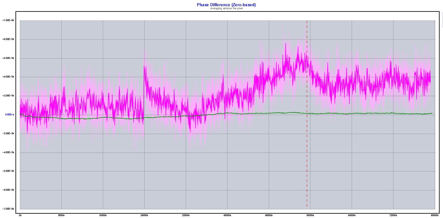
The plot on the left should give an indication. Here I show, in pink, a Ublox 6T PPS compared to the NetRS PPP clock residuals, in green. The PPS of the Ublox is driving the start input on a PM6681 TIC, the stop input is driven by the maser 5MHz signal. Sawtooth correction applied in software. Same oscillator, same antenna, collected at the same time.
I can not overstate the value of a continous measurement of the reference used in stability measurements. I can not count the number of times I have looked at a plot, wondering what caused an anomaly - was it my reference? Or was it the DUT? How do I know? With these measurements in place, it is just a matter of checking. If it was the reference, it will show up in the phase records.
Cookbook
Step 1: Set up the GPS receiver
First, the external 10 MHz signal must be connected to the NetRS. Then, in the "Receiver Configuration"-section on the NetRS web-interface, select External Frequency. The web-interface will indicate if a valid reference is detected. I also had to disable Clock Steering to get the receiver to use the reference.I also should mention that I have not had success with mixed L2C and L2P(Y) observations. I do not know precisely what the issue is, but for now I run my receiver tracking L2P(Y) only. For the NetRS, this is configured in "Reciever Configuration", under "L2-tracking". Set to "L2-Y-code Only".
Next, data logging must be configured. In the "Data Logging"-section, I have defined a Continous logging with 1440 minutes duration, in binex-format. Measurement interval should be no longer than 30 seconds, although I am not convinced much shorter intervals than this gives much benefit.
Ensure the log is enabled and logging, and leave the receiver alone until the next day.
Step 2: Convert the observations to RINEX
To get a RINEX-file from the receiver, download the previous days binex-file with your favourite tool - I use WinSCP, as it is easy to create daily scripts to retrieve (and optionally delete) the observation-files from the receiver.The observations must be converted to a valid RINEX observation-file. I use teqc.exe with the following cmd-line:
teqc.exe -binex +out RINEX-filename +O.at LEIAT502 BINEX-filename
Substitute RINEX-filename and BINEX-filename as appropriate, of course. The +O.at LEIAT502 is necessary in order to encode in the RINEX-file the antenna type used. I happen to use a Leica AT502 - valid antenna types can be found in rcvr_ant.tab.
Step 3: Verify
A convenient way to ensure the setup is sane is to upload the resulting RINEX-file to NrCAN. A free account is required. Process the files in the ITRF reference frame, Static mode.This could be the last step. The resulting report is quite good, and contains pretty much all the information required. PPP Direct, a few trivial lines of code and a scheduled job, and you will have a nice report in your inbox every morning of how your oscillator is doing.
The main drawbacks of this method, in my opinion, is that I have not found a way to make NrCAN do what is known as reverse filtering - in short, the first few hours of the results will be noisy as the Kalman filter converge on the solution - this makes the phase record hard to work with. Also, it is a bit cumbersome to script the receipt of an email with a zip-file.
If you prefer to run the process yourself to get round these limitations, it is a little more involved - but not by much.
Step 4: Download gLab
gLAB is a software tool suite developed under an European Space Agency (ESA) Contract by the research group of Astronomy and Geomatics (gAGE) from the Universitat Politecnica de Catalunya (UPC). Given the RINEX-file and relevant corrections, it will perform the calculations for us. (I use version 5.00 at the time of writing.)I also want to mention here a pair of books available for free on the website that is worth a look: GNSS Data Processing Book
The installation requires nothing more than clicking "next".
Step 5: Download required corrections
In order to make gLab process our RINEX-file, we need the correct .sp3 and .clk-files. Also we need igs08.atx, available here. (This file is not updated frequently, needs refreshing if the station antenna changes or a new satellite comes on line)Step 6: Run gLab and extract the result
The options to gLab can be a bit daunting at first glance. Here is the cmd-line I use:
glab.exe -input:obs rinexfile -input:orb sp3file -input:clk clkfile -output:file outfile -input:ant igs08.atx -pre:setrectype 2 -pre:setrecpos calculate -filter:backward -print:none -print:filter
gLab can also read a config file with options, specify -input:cfg filename. Many of the options will not change from run to run, and can be written in this file to be included in every run.
If all goes well, we now have a temporary file with the output from the filter. It is now a matter of (1) getting the field containing the offset of the local oscillator, multiplying by the speed of light to get the offset in units of time, and (2) ignoring the first half of the output (the forward filtering-part), saving the second part, and reversing the list. We now have a nice phase record of our oscillator.
Anders Wallin has some Python scripts to automate the process here.
I also have some C# code that automates this. See my Github-repository, ParseGlabOutput, to get a phase record from the gLab logs.
Step 7: Next up
So far, this really has been a lightning guide to using PPP for stability measurements of oscillators. My ambition was to have a short and concise guide to get some results - not to be rigorous in every (or indeed any) way. There are many factors to using PPP in this way, which may or may not matter depending on your local oscillator. Ocean tidal loading, receiver and satelliteP1-C1/P2-C2 bias, tuning filters and models and phase slip detectors, and the list goes on.One thing I will mention is how to process several days of observations with gLab, since it is far from intuitive.
- The RINEX-files must be combined, which is easily done with
teqc.exe RINEX1 RINEX2 ... RINEXN > RINEXout - Then the clock-products must be combined. This is a cumbersome manual process; (1) Combine all the relevant .clk-files, in increasing order of time, into a single file. (2) Manually go through the resulting file, and remove all the headers except the first one.
- Do the same to the .sp3-file, but additionally you must update the number of data entries in the first line of the header to reflect the total number of entries in the new file. For a weeks worth of corrections, change 96 to 672.
With that said, another option is to simply process observations in daily batches and combining the resulting phase records. This leads to the well known Day Boundary Discontinuity, basically phase jumps between daily batches. Depending on the level of precision required, I found that removing the phase jumps by looking at the Median Absolute Deviation in frequency gives results that are good enough for my use. That process can be summed up as follows:
- Differentiate the (combined) phase record
- Make a temporary copy of the list, convert to absolute values, sort
- Get the Median
- Identify, and replace with zero, any datapoint in the original list larger than some multiple of the MAD. 5 seems a good startingpoint.
- Integrate the list back into a phase record.
For further reading, I highly recommend a thesis by Jian Yao, Continuous GPS Carrier-Phase Time Transfer. Primarily concerned with the Day Boundary Discontinuity, but explains quite a lot about the whole PPP and time transfer thing.